ML-Classification

📅 Date: April 02, 2024
🔍 Domain: Banking
📊 Topic: Predictive Modeling for Telemarketing Campaigns

🔗 View Full Project Files

🧠 Abstract

This project leverages supervised machine learning classification techniques to predict whether a customer will subscribe to a term deposit during a Portuguese bank’s telemarketing campaign. Using publicly available data from the UCI Machine Learning Repository, the aim is to explore how decision-making can be optimized using AI models like Random Forest, Decision Trees, and Boosted Models.

Key benefits for the bank include:

Enhanced targeting of high-potential clients
Improved marketing efficiency and ROI
Actionable insights on customer behavior

📂 Dataset Overview

Source: UCI Bank Marketing Dataset
Features: 17 (Categorical & Numerical)
Target: Binary (yes or no) — whether a customer subscribed

📈 Exploratory Data Analysis

The following visuals were generated:

Subscription Distribution
Age vs. Subscription
Contact Month vs. Success Rate
Loan Status vs. Subscription
Correlation Heatmap
KDE and Histograms for Continuous Features

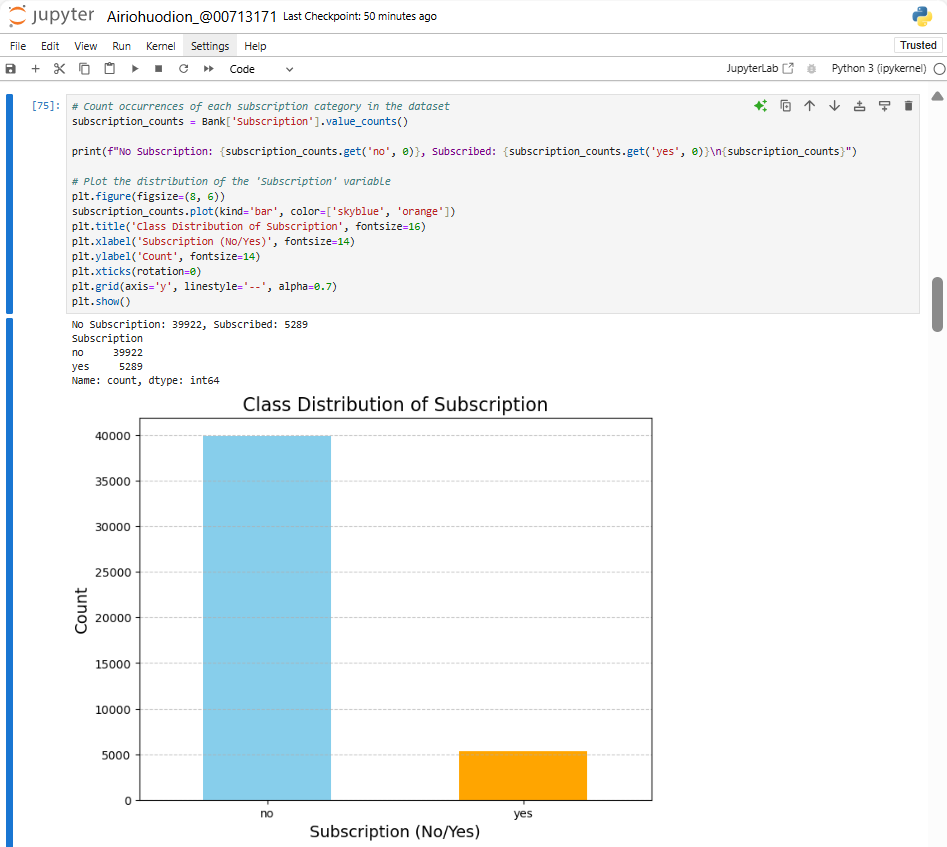Figure 1: Showing the values for No and Yes class on (subscription) target variable.

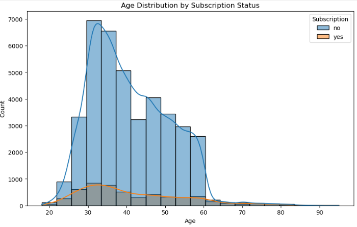subscription status Figure 2: It shows that persons within 30 years subscribe the most.

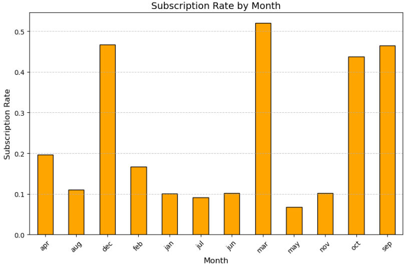subscription per month Figure 3: This code uses a bar chart with stylised formatting to compute and display subscription rates by month. The month of march has highest subscription rates.

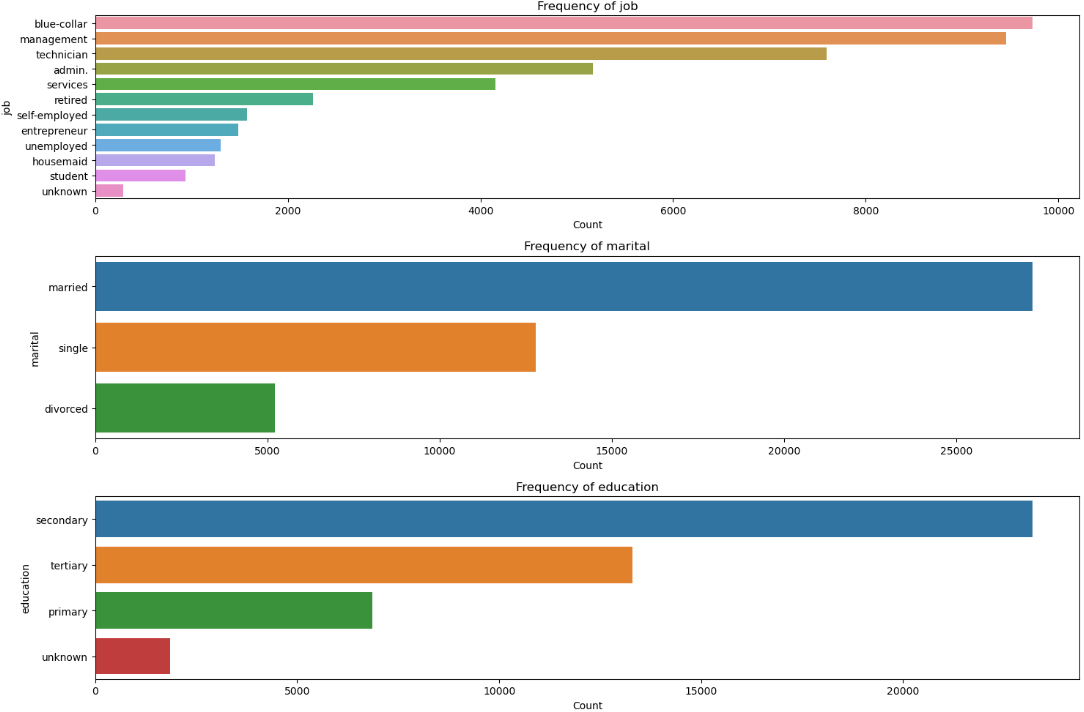frequency of jobs Figure 4:The categorical features analysis shows histograms and KDE plots of the distribution of continuous features.

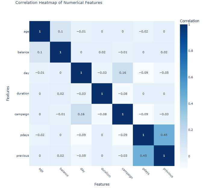correlation heat map Figure 5:Calculated numerical features for correlations, visualising and to view them interactively for insights into relationships.

🔑 Variables

Demographics: age, job, education, marital status
Campaign Details: call duration, contact month, number of contacts
Socio-Economic Indicators: consumer confidence index, employment rate, interest rate

🧹 Data Preprocessing

Categorical Encoding with One-Hot Encoding
Standardization with StandardScaler
Feature selection via RFECV
Class imbalance handled using Random UnderSampling and SMOTE

onehotencoding

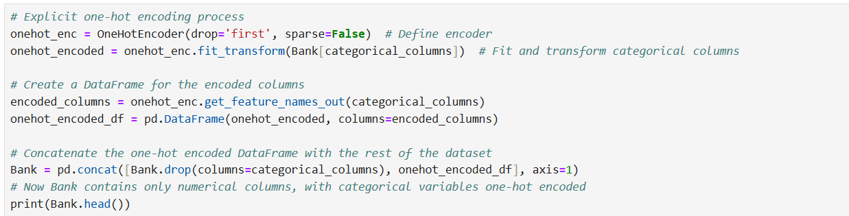
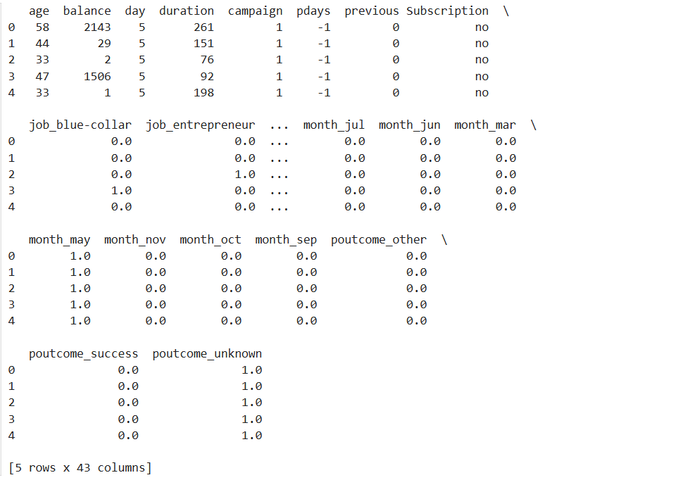onehotencoding Figure 6: Firstly I removed the target variable and deleted the dummy class variables I used for visualisation. The dataset categorical variables are fully encoded as one-hot-encoded features and ready for modelling.

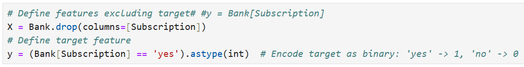
spliting Figure 7: Above I defined my features and target, I then converted my target “y” from (yes to 1 and no to 0) Splitting all feature into ‘X’ and target variable to ‘y’

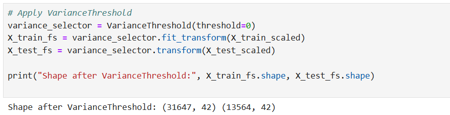Figure 8: From the result, no features were removed this means all training and testing sets had variance above the threshold.

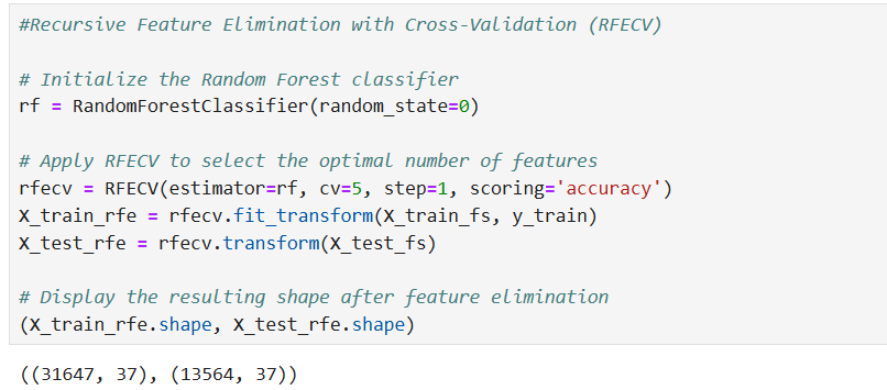RFselection Figure 9: The result “((31647, 37), (13564, 37))” shows that the feature selection process reduced the dataset from 42 to 37 features. This means 5 features were identified as less important and removed, leaving a more focused set of features for the model. This will make the model more efficient and potentially improve its performance by removing irrelevant or redundant information.

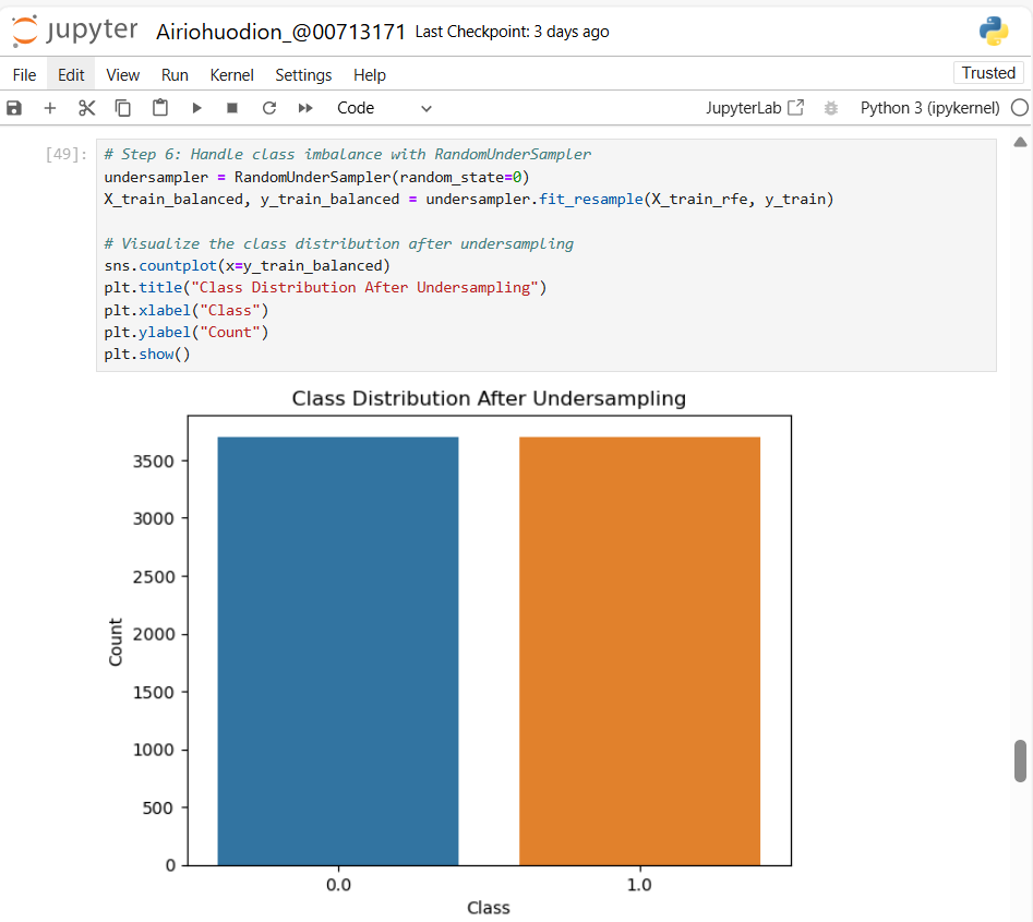undersampled class Figure 10: Addressing class imbalance by applying Random Undersampling, balancing the dataset target variable for improved model fairness.

🤖 Models Implemented

1️⃣ Decision Tree Classifier

Accuracy: 80.3%
Issues: Poor recall on the minority class
Tuned Accuracy: 82.3%

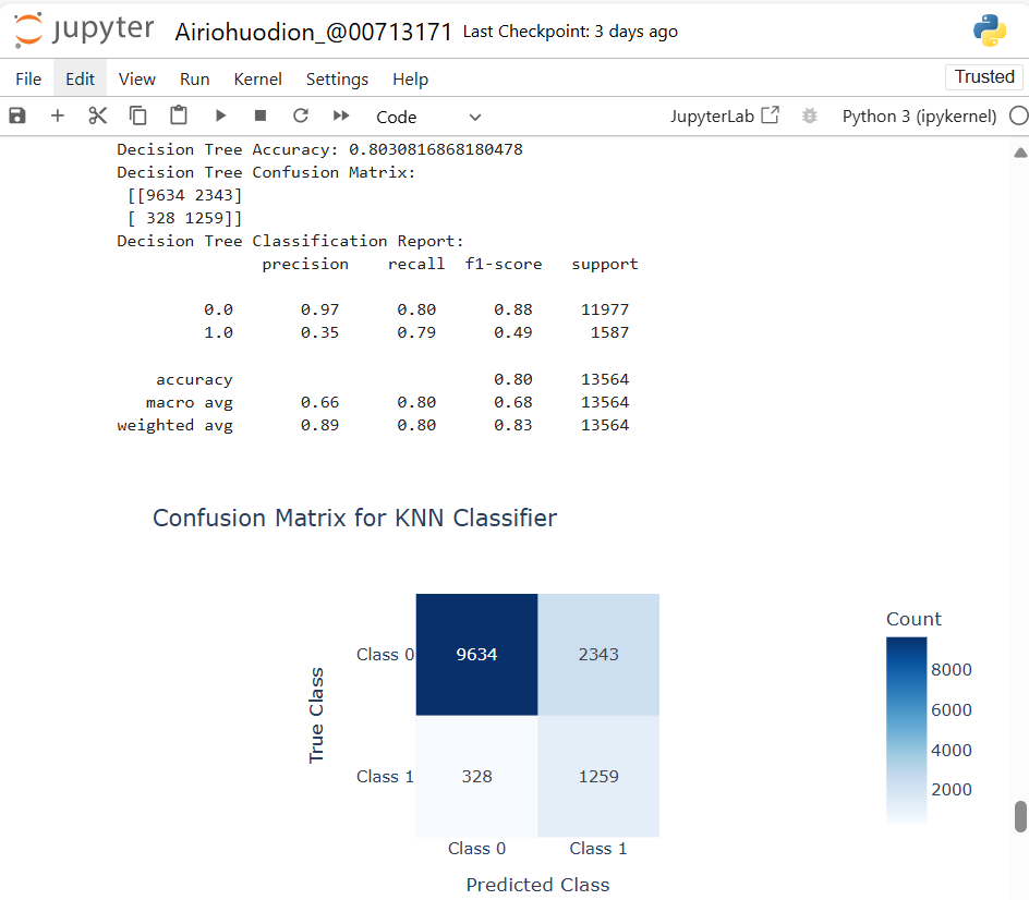Figure 11: The Decision Tree Classification result reports 80% accuracy and the confusion matrix is as follows.

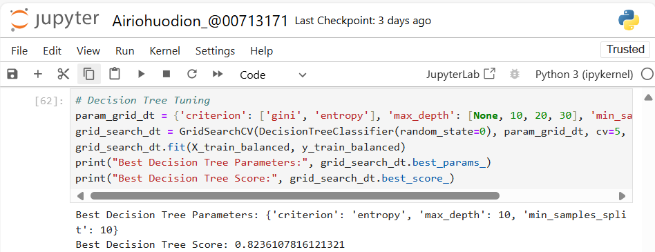decission tree tune Figure 12: The best cross-validated accuracy achieved with these parameters is 82.36%, indicating improved performance compared to the untuned model. This configuration balances complexity and predictive accuracy, making it more robust.

2️⃣ Random Forest Classifier

Accuracy: 83.0%
Tuned Accuracy: 86.1%
Strengths: Strong performance on minority class, better generalization

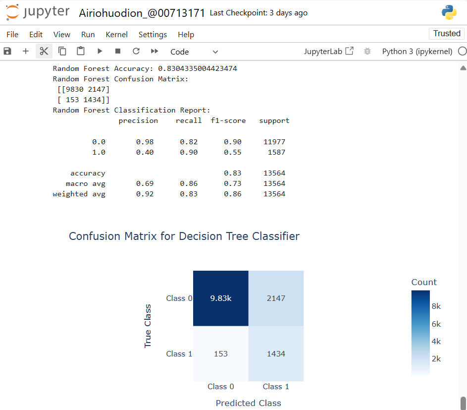randomforestclass Figure 13: The Random Forest classifier achieved an accuracy of 83.04%. The Random Forest performs better on minority Class 1 compared to Decision Tree but still struggles with precision, indicating room for improvement in predicting positive cases.

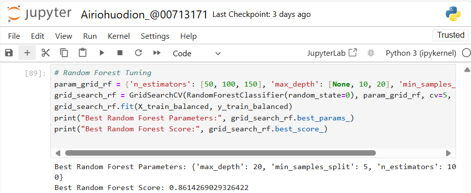RFtune Figure 14: The best cross-validated accuracy achieved is 86.14%, demonstrating improved performance with the tuned parameters. This setup balances complexity and predictive power for robust model performance.

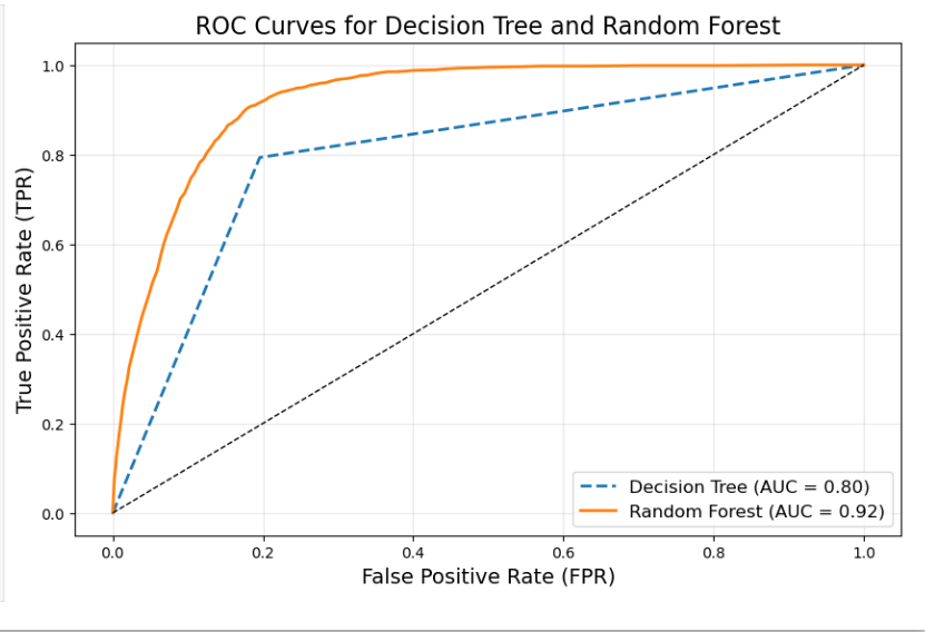ROC_Curve Figure 15: The outcome above distinguishes the positive and negative class using “Area Under the Curve(AUC)”

3️⃣ Azure ML Boosted Decision Tree

AUC: 0.94
Accuracy: 90.8%

4️⃣ Azure ML Neural Network

AUC: 0.906
Accuracy: 89.7%

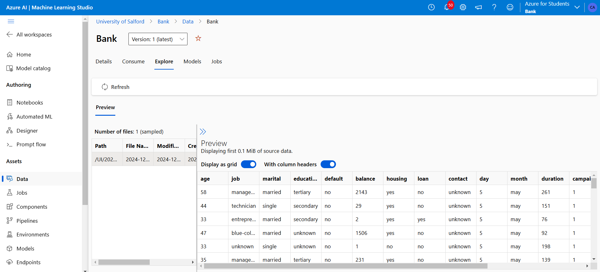Azure Dataset Upload Figure 15: Dataset upload into Azure table and visualisation

Convert to Indicator Values - Step 1

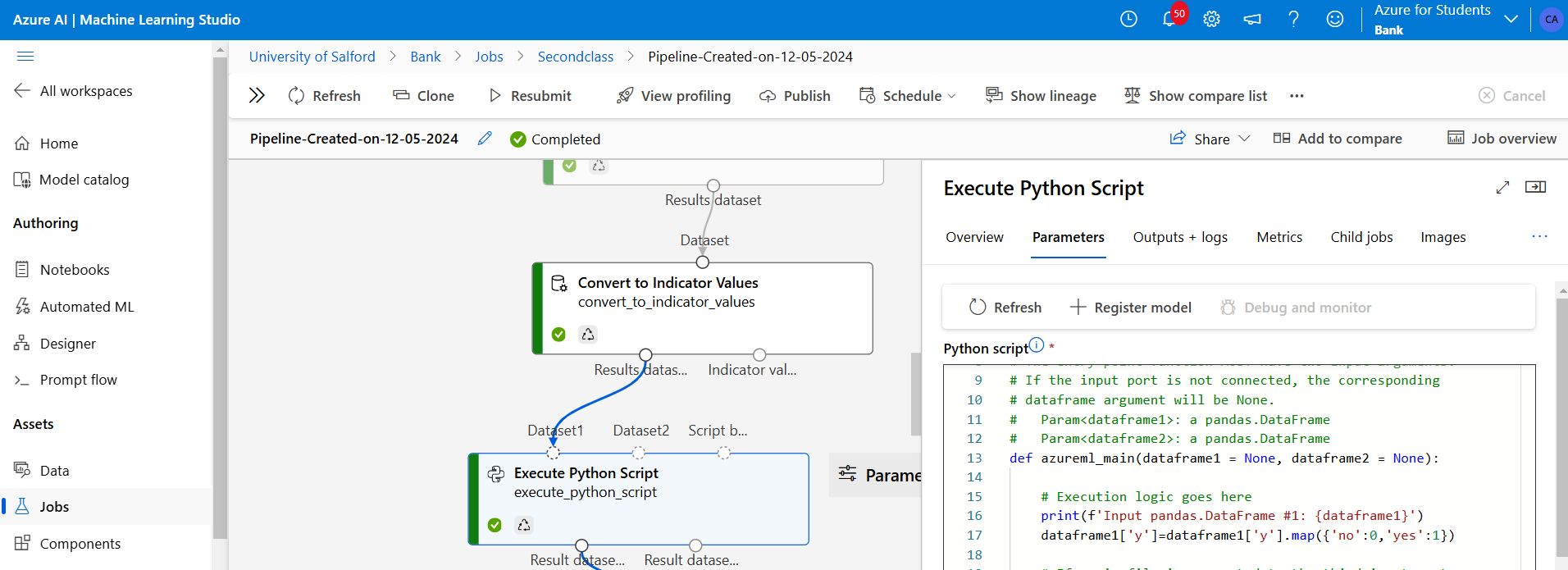
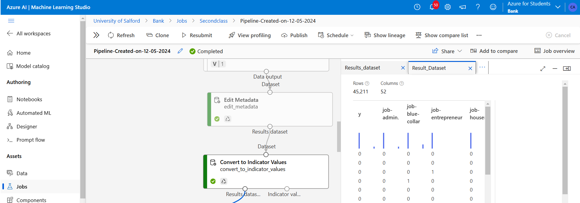
Figure 16: Using Execute-Python-Script was used to convert the categorical target variables from (yes to 1 and no to 0).

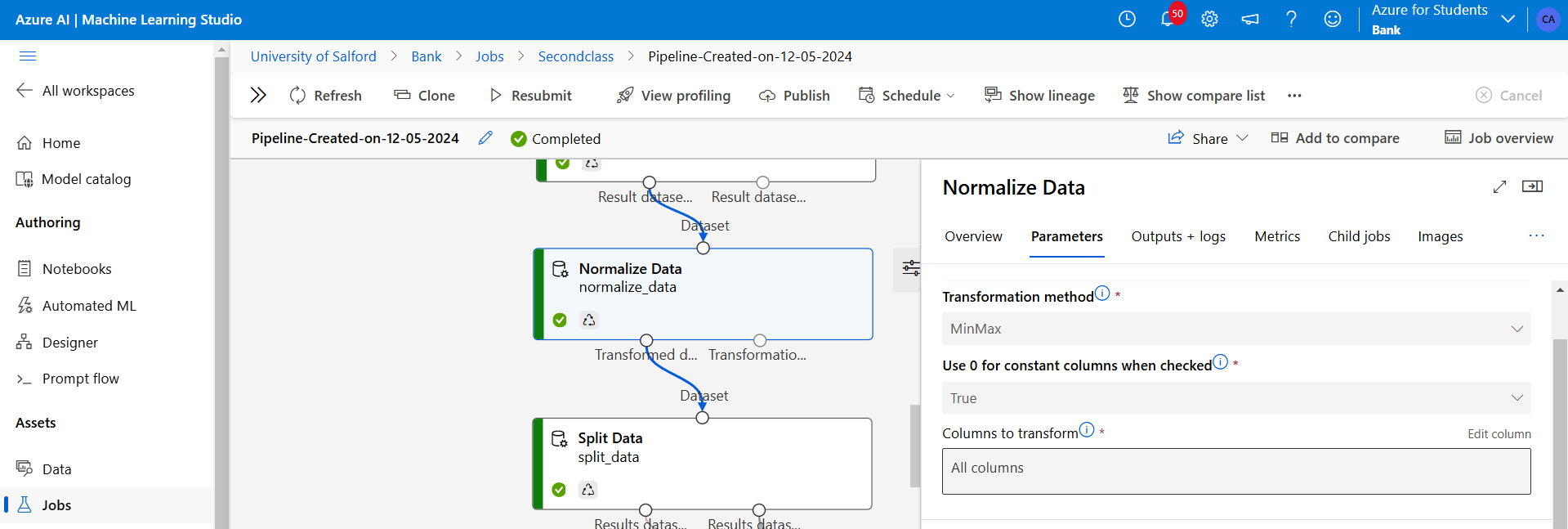
Figure 17: Using the normalise data module above to scale the dataset using MinMax scaler method.

transformeddata
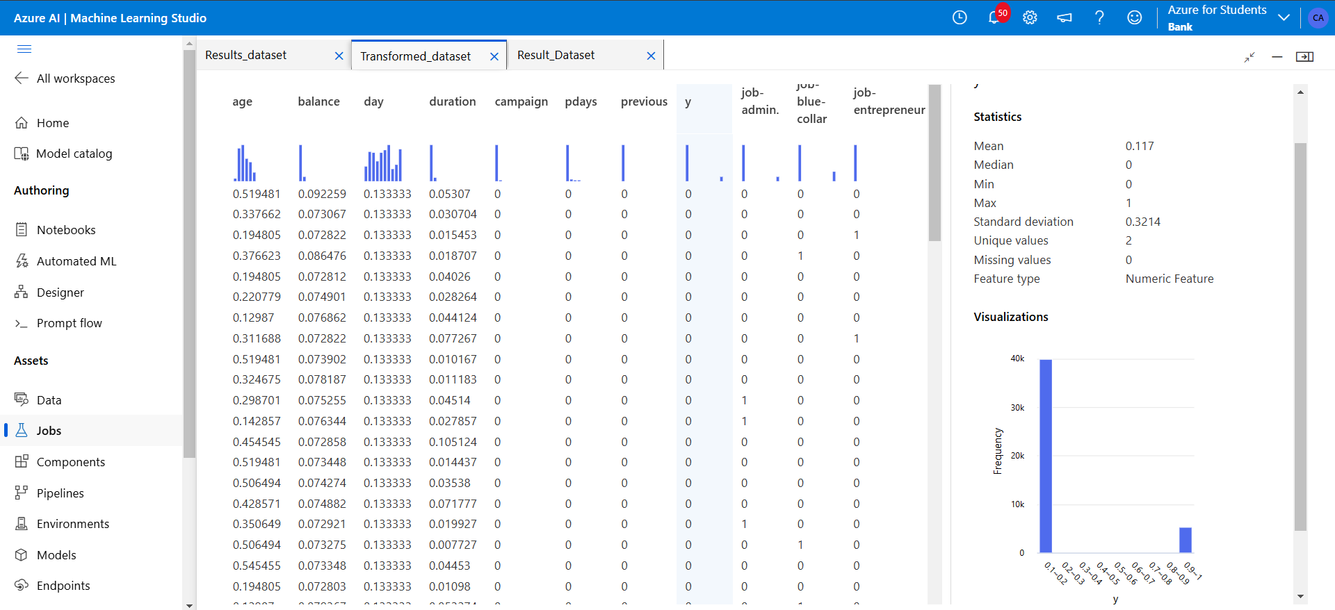
Figure 18: Next above, is shown the imbalanced class label “y” where 1 is highly dominated by 0.

smotetarget
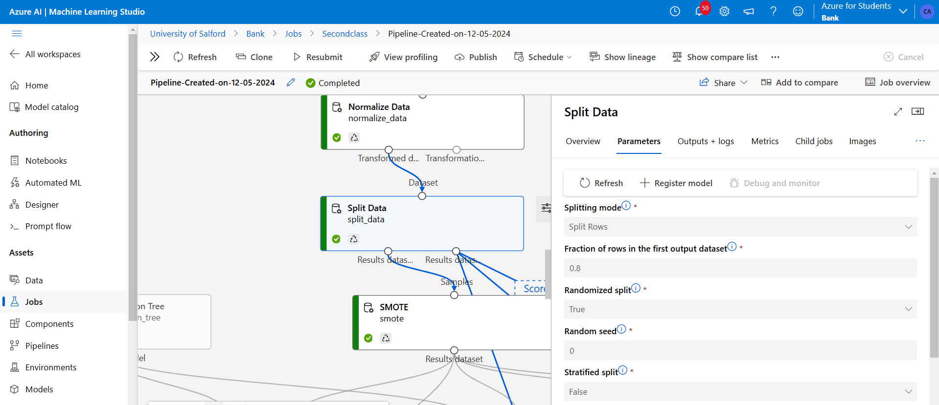
Figure 19: Next above, I split the result into 80% training and 20% testing and then I carried out SMOTE to improve the balancing of “y” also known as subscription.

azuretune
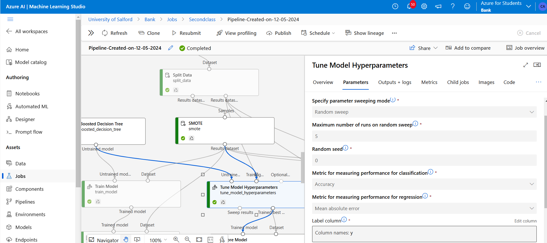
Figure 20: Also above I have attached my Two-class-boosted Decision Tree to Tune Model Hyperparameters which trained the tuned version of the model, then it would output the most efficient combination by accuracy, and compared to base model.

first half
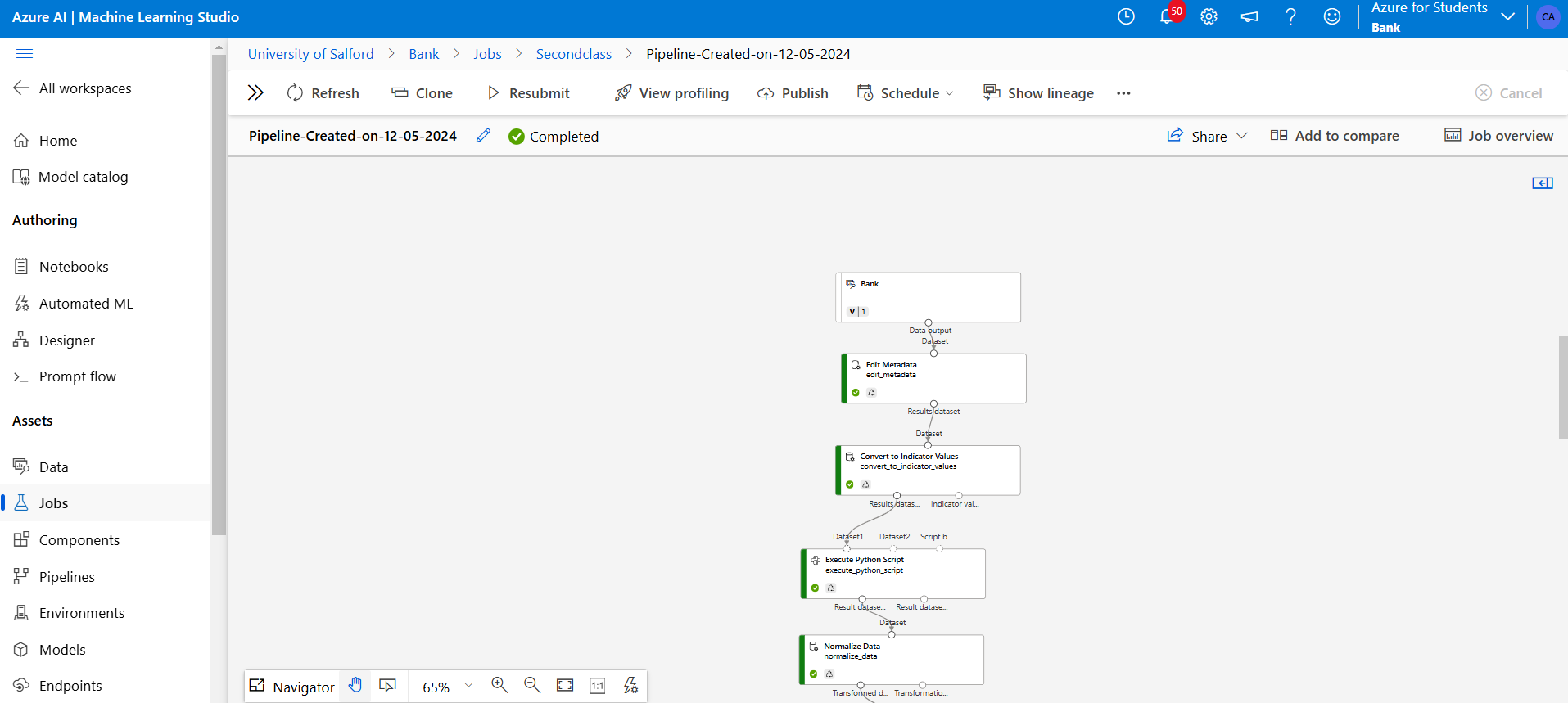
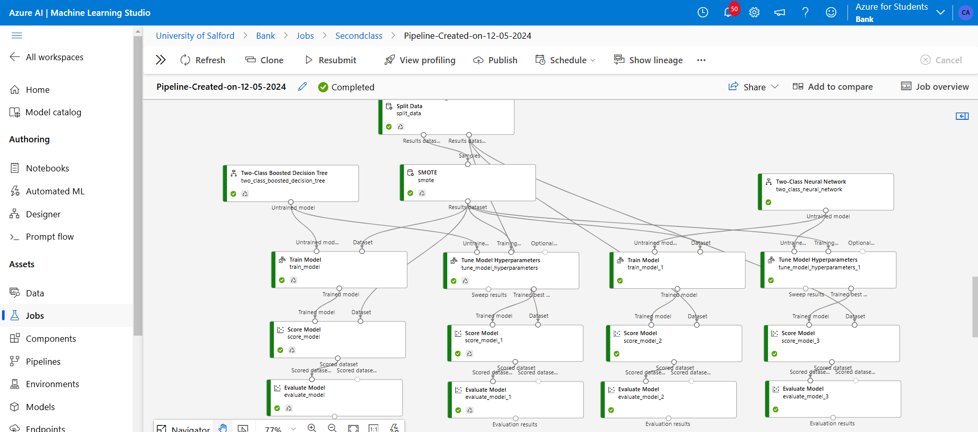finalhalf Figure 21: The Score model follows and the Evaluate model are added to generate and analyse model performance.

📊 ROC Curve Visual

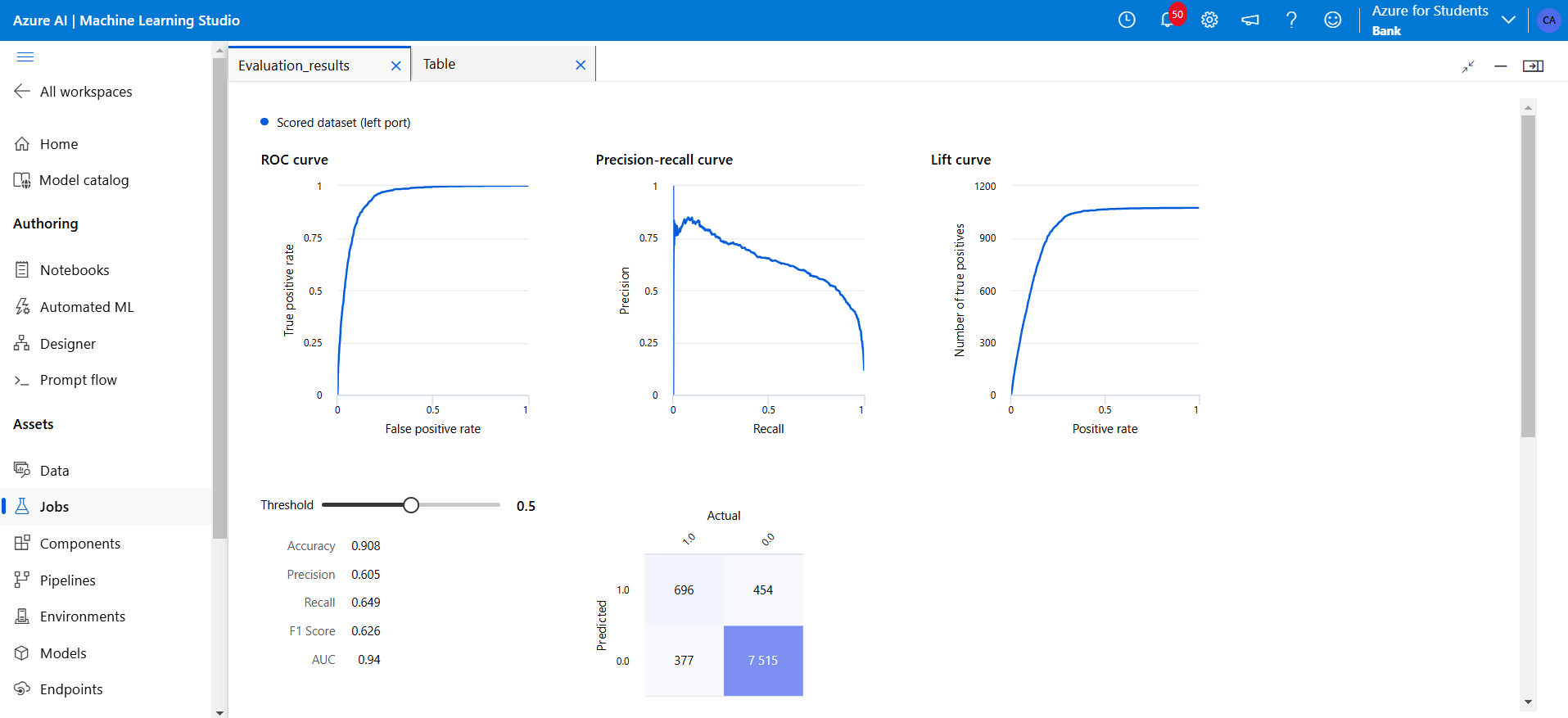azuretwoclass Figure 22: This shows the Two Class Boosted Decision Tree Report

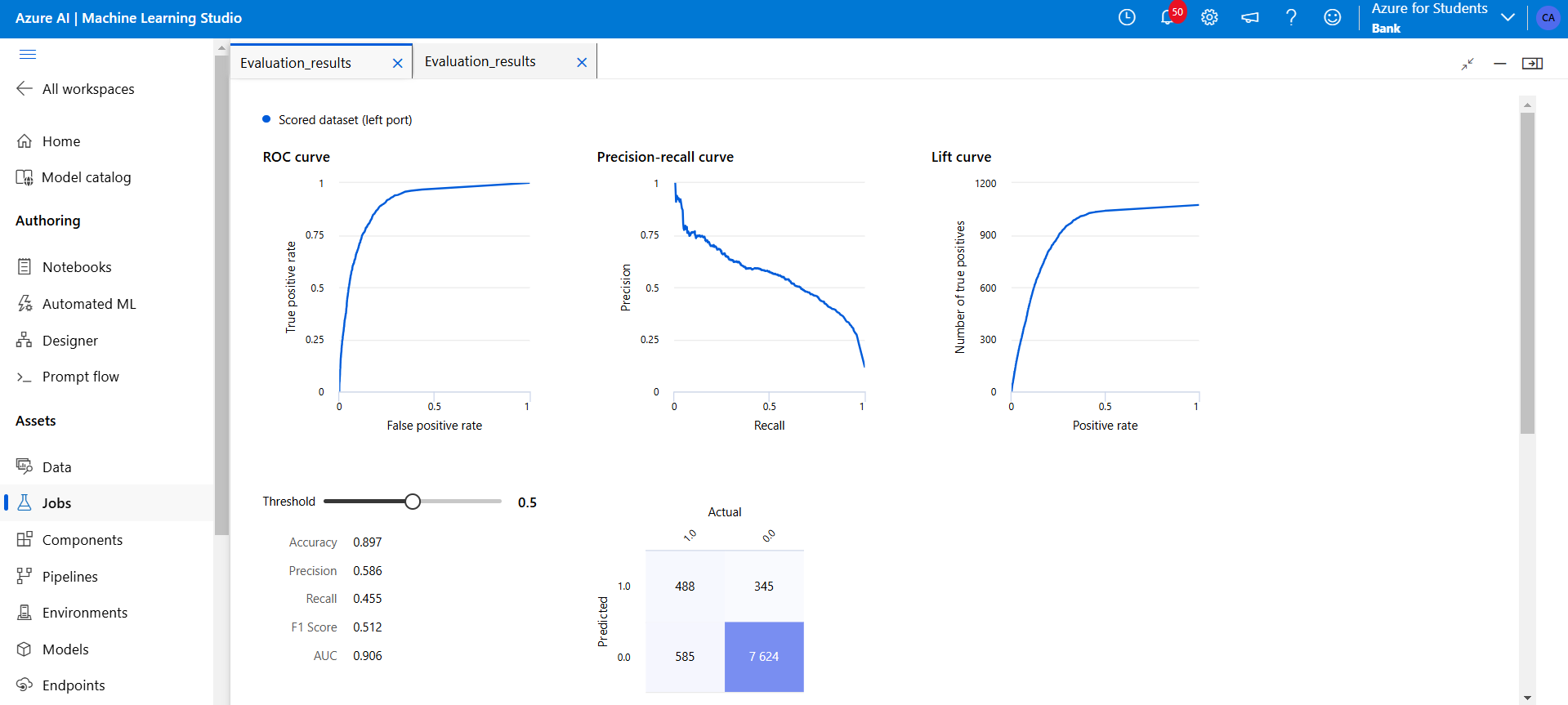twoclassneural Figure 23: This shows the Two-Class Neural Network.